Query Performance Optimization Guide
Download
Focus Mode
Font Size
Foreword
To enhance task execution efficiency, you can first perform insight analysis on existing tasks or engines (Spark only) to check whether there is adjustable space. Followed by DLC, which has many optimization measures during the computation process, such as data governance, Iceberg indexing, and cache. You can combine these optimization measures to further optimize tasks. Using them correctly can not only reduce unnecessary scan cost but even improve efficiency by several or even dozens of times.
Here are some optimization ideas at different levels.
Spark
Task Insights
Based on various Metrics collected by the Spark engine, the Task Insight module implements algorithms to automatically analyze Metrics, offering task insights. It is advisable to implement based on recommended parameters and optimization solutions.
It can address common SQL issues, including:
Resource Preemption
Data skew
Insufficient disk space or memory OOM
Slow Task
Too many small files
Unreasonable Shuffle
Execution Plan Analysis
When task insight still cannot meet performance tuning, further analysis of SQL bottlenecks can be conducted based on the execution plan of the current task provided by Spark UI.
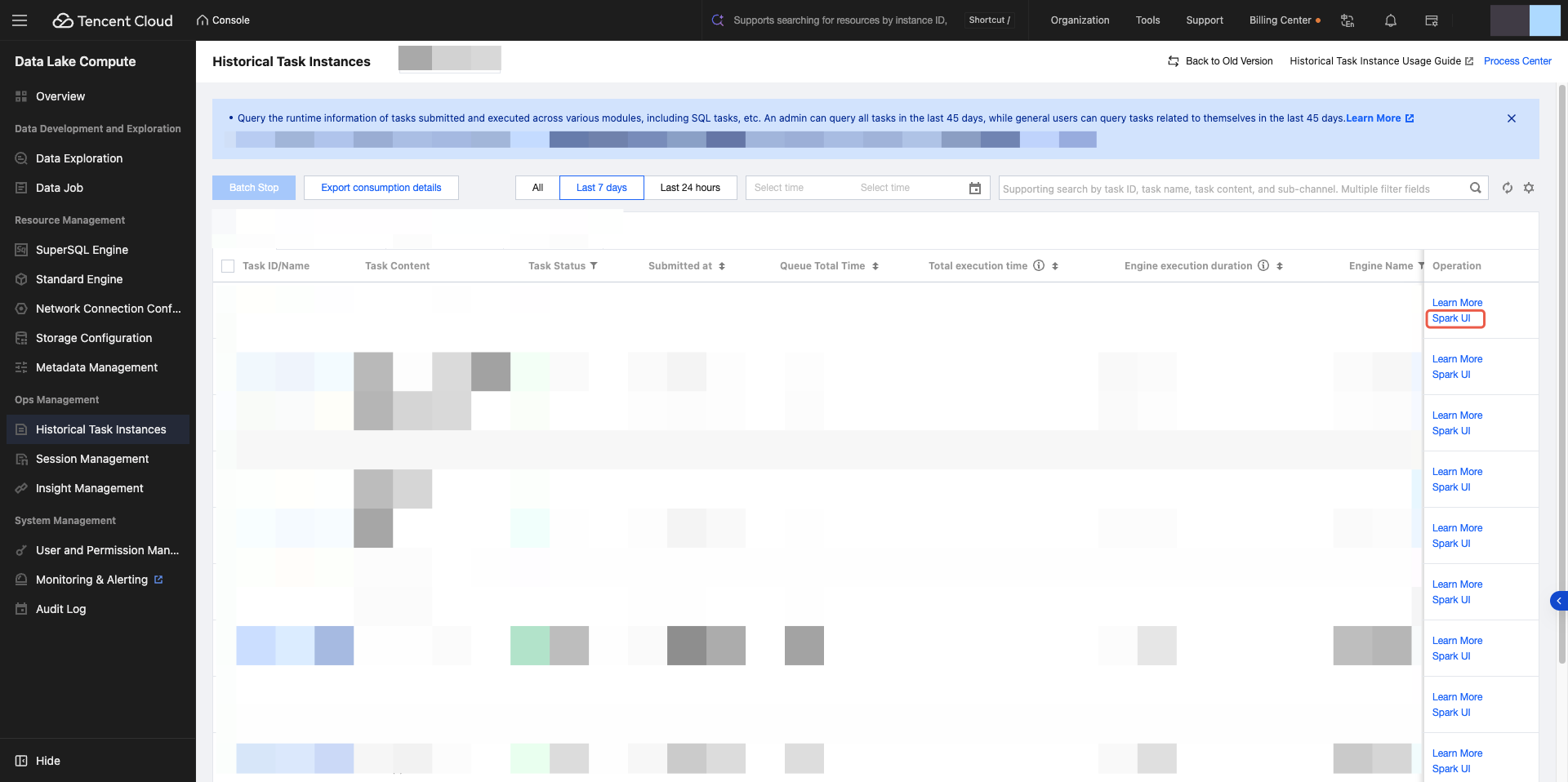
Spark UI allows you to view the execution plan from the SQL DataFrame page.
View and analyze the execution plan by combining the Stage duration on the Stages page according to the steps below and optimization idea. Before optimization, it is advisable to have a preliminary judgment on the data magnitude of input, Join, and output in advance.
Step 1: Analyze the Scan Operator
The Scan operator is responsible for reading all database tables. The Stages page contains the Stage with Input data, which generally corresponds to the Scan operator. When this kind of Stage is time-consuming, focus on viewing the Scan operator metrics.
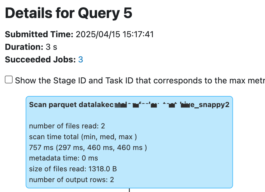
The following metric names vary between Hive and Iceberg tables, however the metric content and meaning are basically the same.
Number of files read: If too many files are read and the size of files read/number of output rows is too small, it can be considered that there are too many small files. Merge small files or use Enabling Data Optimization to configure automatic merging.
scan time total (min, med, max): time distribution when reading distributed. If some tasks read too slowly, it may be because of traffic throttling or rate limiting on the storage COS bucket. We recommend checking the COS bucket monitor and submitting a ticket to adjust bandwidth.
size of files read: Helps determine whether the amount of data read is reasonable. If a file too large is detected, determine whether the stored file format is wrong or dirty data exists.
number of output rows: Helps determine whether the amount of data read is reasonable. If the amount of data read is too large, combine with the Scan Filter criteria to determine whether an error in the Filter condition caused a full table Scan. The Spark engine can automatically push down Filter conditions to the Scan operator. However, if specific special cases do not automatically push down Filter conditions, you can push down the where clause in the SQL in advance.
Step 2: Search for the Bottleneck in Calculation
It is advisable to first view the StageId that takes the longest time to execute on the Stages page, then analyze the execution plan based on the StageID (check Show the Stage ID and Task ID on the page).
Task insight helps identify common performance bottlenecks, while execution plan analysis often requires combining the context of bottleneck operators.
Project operator
Project operators often require attention to whether there is a large number of duplicate Expression definitions. It is advisable to rewrite the SQL to avoid repeated calculation.
Filter operator
Filter operators should generally check if the filter criteria correctly filter data, with a key focus on whether there is a normal reduction in data volume before and after the filter.
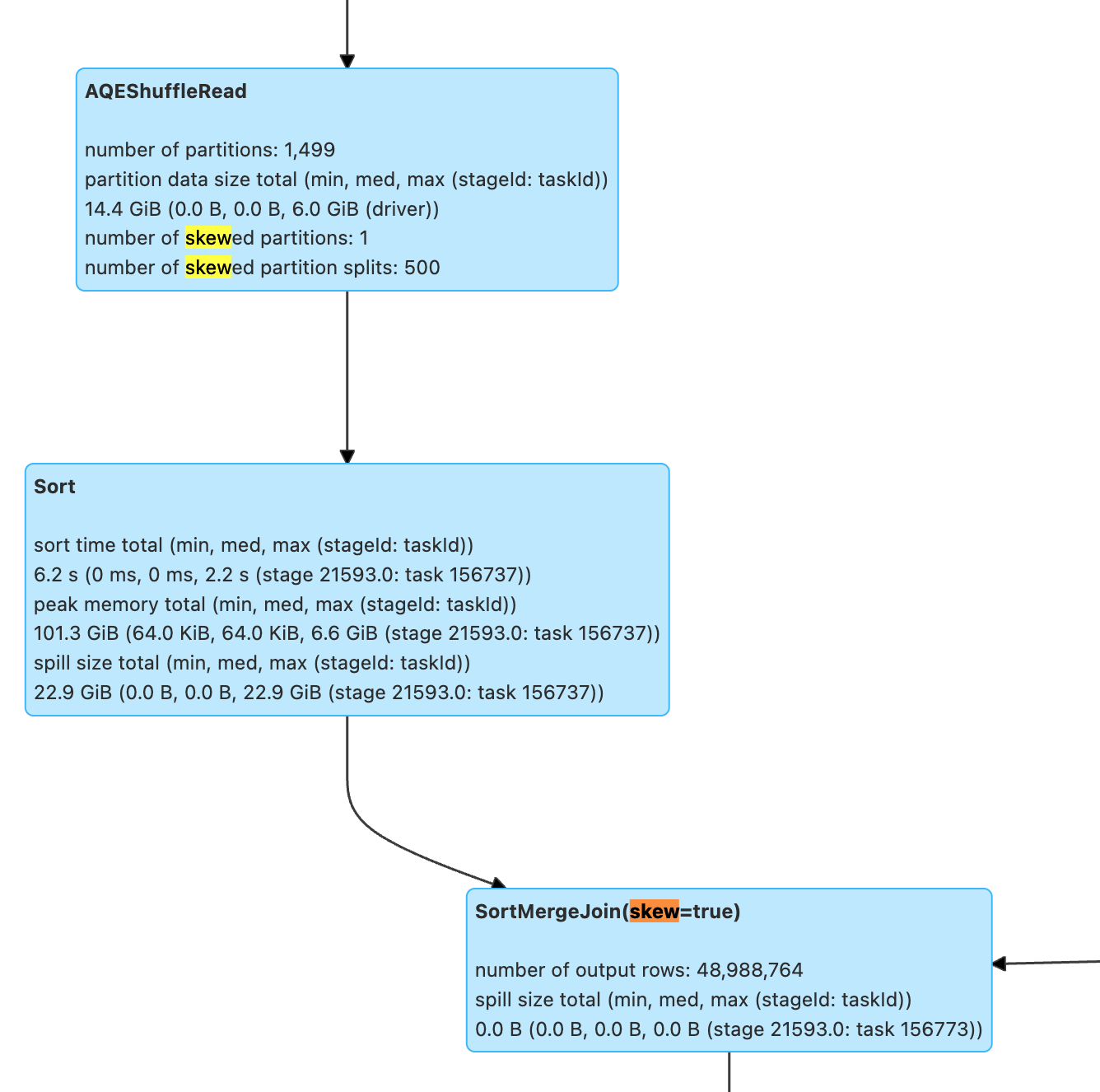
Join operator
Join is a relatively common operator where performance bottlenecks occur. Common optimization ideas are as follows.
SortMergeJoin encounters skewJoin. Although Spark will optimize skewed joins by default, performance will sharply decline once spill occurs when the data inflation coefficient is small (spark.sql.adaptive.skewJoin.skewedPartitionFactor=5.0, exceeding 5 times the mean is considered skewed) or when the skew is not especially prominent (spark.sql.adaptive.skewJoin.skewedPartitionThresholdInBytes=256MB, larger than 256MB is considered skewed). There is still some room for tuning.
SortMergeJoin data volume too large, combine SQL and execution plan analysis:
1. Whether a Cartesian product is displayed, duplicate condition fields in join on cause data inflation in left join or inner join.
2. Are some filter conditions not pushed down, for example, Aggregate operations may block the pushdown of filter conditions. Set spark.sql.optimizer.AggregatePushdownThroughJoins.enabled=true to check whether the operators after Aggregate can be pushed down.
SortMergeJoin encounters large table join small table. Is it possible to replace with BroadcastHashJoin? Use Spark hints or increase spark.sql.autoBroadcastJoinThreshold=10MB to allow the small table to broadcast.
Aggregate operator
Aggregate commonly has a skew problem. When there are too many Aggregate keys, it can cause slow tasks. If adjusting the number of partitions does not resolve the skew, it can only be achieved by readjusting the keys to distribute the excessive keys and redesign the business SQL. In addition, if the function in Aggregate has repeated calculation, you can also consider simplifying it at the SQL level.
Exchange + AQEShuffleRead operator
AQE is a feature provided by Spark to automatically merge too small partitions and split oversized partitions during shuffle. The above Join/Aggregate often requires checking the Exchange+AQEShuffleRead operator. AQE determines the partition size during ShuffleRead based on spark.sql.adaptive.advisoryPartitionSizeInBytes=64MB. Therefore, when business data inflation occurs significantly, such as small data volume join generating very large data amount, you can consider reducing the advisory partition size. Or when the data volume shrinks significantly after Shuffle processing, you can consider increasing the advisory partition size to avoid too many small files.
Step 3: View the Insert/Write Operator
The Stages webpage contains Output Stages, which can correspond to write operators.
General tasks usually end with write operators such as Insertxxx, Overwritexxx, or AppendData. Attention required for whether there is too many small files and the time when commit occurs.
Common metric meanings:
number of output rows: whether the amount of data written meets expectations, especially when there is a significant performance change, attention required.
task/job commit time: After data write, commit is required to confirm the correctness of the entire table's data. If commit takes too long, it is usually due to the rename operation in a normal bucket. You can consider switching to a metadata acceleration bucket or submit a ticket for COS bucket consultation.
number of dynamic part: By default, dynamic partition write is enabled. If there is only one partition written, check whether there is an Exchange operator before the write operator that partitions on a field with only one value, which can cause distributed write to change into single-thread write. For Hive table write, you can adjust the partition policy when writing through Spark hints; for Iceberg table, adjust `spark.sql.iceberg.distribution-mode`=none.
Presto
Optimize SQL Statements
Scenario: The SQL statement itself is unreasonable, leading to poor execution efficiency.
Optimize JOIN Statements
When a query involves JOINs with multiple tables, the Presto engine prioritizes completing the JOIN operation for the table on the right side of the query. Generally, completing the JOIN for the smaller table first, then joining the result set with the larger table, leads to higher execution efficiency. Therefore, the order of JOINs directly affects the query's performance. DLC Presto automatically collects statistics for inner tables and uses CBO to reorder the tables in the query.
For outer tables, users can usually collect statistics through the analyze statement or manually specify the order of JOINs. If manual specification is needed, please order the tables by size, placing the smaller table on the right and the larger table on the left, as in tables A > B > C, for example: select * from A Join B Join C. It is important to note that this does not guarantee increased efficiency in all scenarios, as it actually depends on the size of the data set resulting from the JOIN.
Optimize GROUP BY Statements
Arranging the order of fields in the GROUP BY statement can improve performance to a certain extent. Please sort the aggregation fields by cardinality from highest to lowest, for example:
// Efficient approachSELECT id,gender,COUNT(*) FROM table_name GROUP BY id, gender;// Inefficient approachSELECT id,gender,COUNT(*) FROM table_name GROUP BY gender, id;
Another optimization method is to use numbers to replace the specific grouping fields as much as possible. These numbers represent the positions of the column names following the SELECT keyword, for example, the above SQL can be replaced as follows:
SELECT id,gender,COUNT(*) FROM table_name GROUP BY 1, 2;
Use Approximate Aggregate Functions
For query scenarios that can tolerate a small amount of error, using these approximate aggregate functions can significantly improve query performance.
For example, Presto can use the APPROX_DISTINCT() function instead of COUNT(distinct x), and the corresponding function in Spark is APPROX_COUNT_DISTINCT. The drawback of this approach is that approximate aggregate functions have an error margin of about 2.3%.
Use REGEXP_LIKE instead of multiple LIKE statements
When there are multiple LIKE statements in SQL, you can often use regular expressions to replace multiple LIKEs, which can significantly improve execution efficiency. For example:
SELECT COUNT(*) FROM table_name WHERE field_name LIKE '%guangzhou%' OR LIKE '%beijing%' OR LIKE '%chengdu%' OR LIKE '%shanghai%'
Can be optimized to:
SELECT COUNT(*) FROM table_name WHERE regexp_like(field_name, 'guangzhou|beijing|chengdu|shanghai')
Data Governance
Data Governance Use cases
Scenario: Real-time writing. Flink CDC real-time writing usually adopts the upsert method, which generates a large number of small files during the writing process. When small files accumulate to a certain extent, it can cause data queries to slow down, or even result in timeout failures.
You can check the number of table files and snapshot information in the following way.
SELECT COUNT(*) FROM [catalog_name.][db_name.]table_name$files;SELECT COUNT(*) FROM [catalog_name.][db_name.]table_name$snapshots;
For example:
SELECT COUNT(*) FROM `DataLakeCatalog`.`db1`.`tb1$files`;SELECT COUNT(*) FROM `DataLakeCatalog`.`db1`.`tb1$snapshots`;
When the number of table files and snapshots is excessive, refer to the document Enable data optimization to activate the data governance feature.
Data Governance Effectiveness
After enabling data governance, there was a significant improvement in query efficiency. For example, the table below compares the query time before and after merging files. The experiment used a 16CU Presto, with a data volume of 14M, 2921 files, and an average of 0.6KB per file.
Executed Statement | Merge Files | Number of files | Number of records | Query time consumption | Effect |
SELECT count(*) FROM tb | No | 2921 items | 7895 entries | 32s | 93% faster speed |
| SELECT count(*) FROM tb | Yes | 1 item | 7895 entries | 2s |
Partition
Partitioning enables the classification and storage of related data based on column values with different characteristics such as time and region. This significantly reduces scan volume and improves query efficiency. For more details on DLC external table partitioning, please refer to Quick Start with Partition Table. The table below shows a comparison of query time consumption and scan volume between partitioned and unpartitioned states in a single table with a data volume of 66.6GB, 1.4 billion data records, and an ORC data format. Within it,
dt is a partition field containing 1,837 partitions.Query statement | Unpartitioned | Partition | Time Consumption Comparison | Scan Volume Comparison | ||
| | | Time Consumption | Scan Volume | Time Consumption | Scan Volume |
SELECT count(*) FROM tb WHERE dt='2001-01-08' | 2.6s | 235.9MB | 480ms | 16.5 KB | 81% Faster | Reduce by 99.9% |
SELECT count(*) FROM tb WHERE dt<'2022-01-08' AND dt>'2001-07-08' | 3.8s | 401.6MB | 2.2s | 2.8MB | Faster by 42% | Reduce by 99.3% |
As can be seen from the above table, partitioning can effectively reduce Query Latency and Scan Volume, but Excessive partitioning may backfire. As shown in the table below.
Query statement | Unpartitioned | Partition | Time Consumption Comparison | Scan Volume Comparison | ||
| | | Time Consumption | Scan Volume | Time Consumption | Scan Volume |
SELECT count(*) FROM tb | 4s | 24MB | 15s | 34.5MB | Slower by 73% | 30% More |
It is recommended to filter partitions in your SQL statements using the WHERE keyword.
Cache
In today's trend of Distributed Computing and Compute-Storage Separation, accessing Metadata and Huge Data through Network will be restricted by Network I/O. DLC significantly reduces Response Latency by defaulting to the following Caching Technologies, without the need for your intervention.
Alluxio: Is a Data Orchestration Technology. It provides a Cache, moving data from the Storage Layer to a location closer to Data-Driven Applications, making it more accessible. Alluxio's Memory-First Hierarchical Architecture allows data access to be several orders of magnitude faster than existing solutions.
RaptorX: Is a Linker for Presto. It runs on top of storage like Presto, providing Sub-Second Latency. The goal is to offer a Unified, Cost-Effective, Rapid, and Scalable solution for OLAP and Interactive Use Cases.
Result Cache: Caches the same repeated queries, greatly improving speed and efficiency.
The DLC Presto engine by default supports Tiered Cache with RaptorX and Alluxio, effectively reducing latency in similar task scenarios within a short period. Both Spark and Presto engines support Result Cache.
The following table shows TPCH benchmark data in a total data volume of 1TB Parquet files, using 16CU Presto for this test. Since the test focuses on the caching feature, it primarily selects SQLs with significant IO consumption from TPCH. The tables involved mainly include lineitem, orders, customer, etc. The SQLs involved are Q1, Q4, Q6, Q12, Q14, Q15, Q17, Q19, and Q20. The horizontal axis represents the SQL statement, and the vertical axis represents the running time (in seconds).
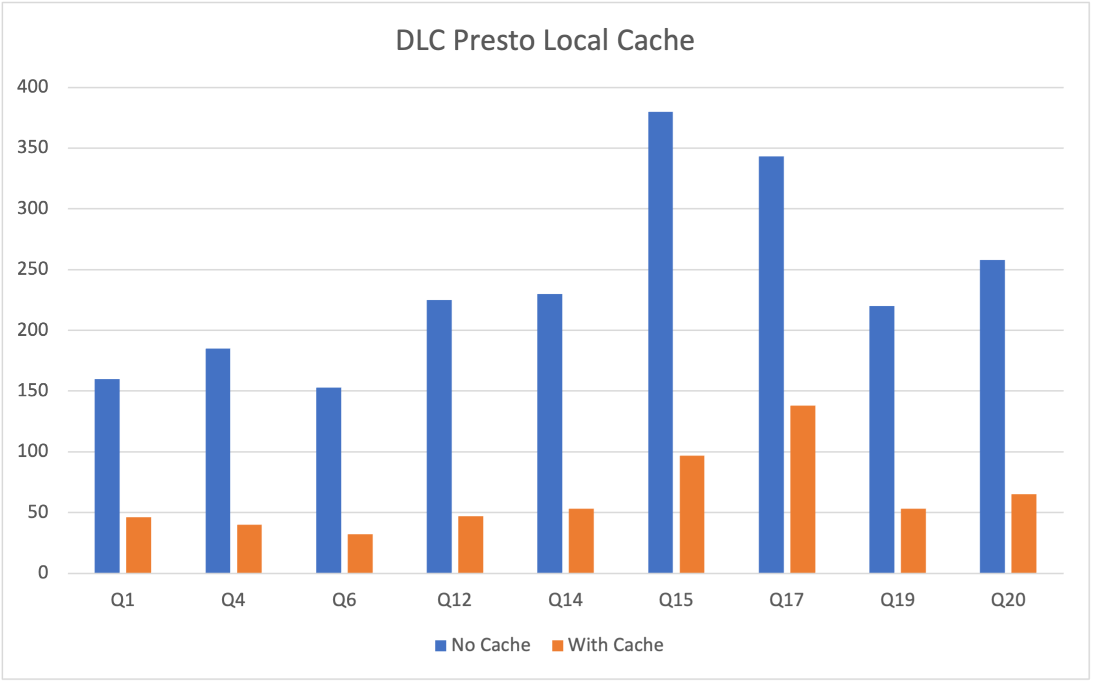
It's important to note that the DLC Presto engine dynamically loads the cache based on Data Access Frequency. Therefore, cache hits cannot be achieved during the engine's first task execution after startup, leading to initial performance still being limited by network IO. However, this limitation is significantly mitigated as the Number of executions increases. The table below shows a performance comparison of three queries in a Presto 16cu cluster.
Query statement | Query | Time Consumption | Data Scan Volume |
SELECT * FROM table_name WHERE udid='xxx'; | First Query | 3.2s | 40.66MB |
| Second Query | 2.5s | 40.66MB |
| Third Query | 1.6s | 40.66MB |
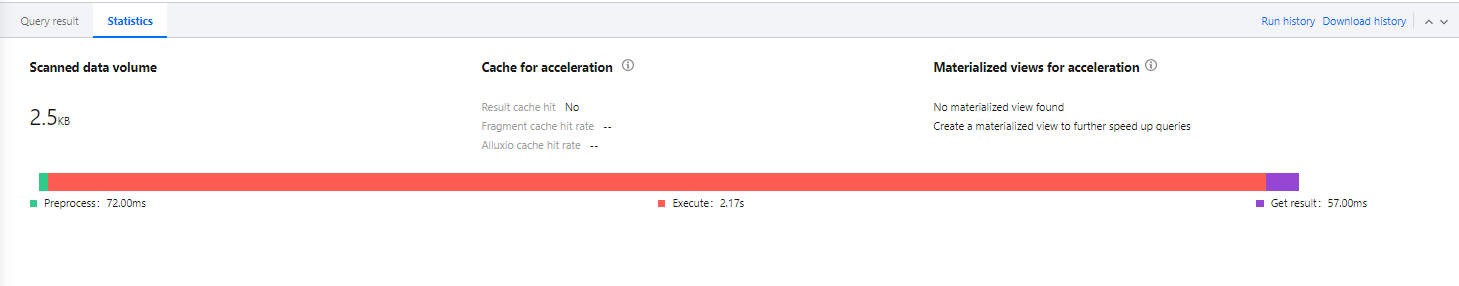
You can view the cache hit ratio of executed SQL tasks in the 'Data Exploration' feature of the DLC Console.
Index
Compared to external tables, the table creation method using internal tables + indexes will significantly reduce both time and scan volume. For more detailed information about creating tables, please refer to Data Table Management.
After creating a table, build an index before inserting based on the business usage frequency, after WRITE ORDERED BY for the indexed fields.
alter table `DataLakeCatalog`.`dbname`.`tablename` WRITE ORDERED BY udid;
The table below shows a comparison of query performance on external and internal tables (with indexes) in a Presto 16cu cluster
Table Types | Query | Time Consumption | Data Scan Volume |
Exterior | First Query | 16.5s | 2.42GB |
| Second Query | 15.3s | 2.42GB |
| Third Query | 14.3s | 2.42GB |
Inner Table (Index) | First Query | 3.2s | 40.66MB |
| Second Query | 2.5s | 40.66MB |
| Third Query | 1.6s | 40.66MB |
It is evident from the table that, compared to external tables, the table creation method using inner tables + indexes significantly reduces both time and scan volume. Moreover, due to cache acceleration, the execution time will also decrease as the number of executions increases.
Synchronous Query and Asynchronous Query
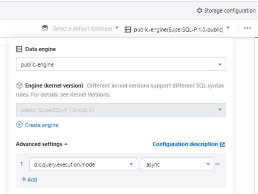
DLC has undergone special optimization for BI scenarios. It can be set to synchronize mode or asynchronous mode (supports only the Presto engine) by configuring the engine parameter dlc.query.execution.mode. The value descriptions are as follows.
async (default): In this mode, tasks complete full query calculations, and the results are saved to COS before being returned to the user, allowing users to download the query results after the query has completed.
sync: Under this mode, it is not necessary to perform full calculation. Once partial results are available, they are directly returned to the user by the engine, without being saved to COS. Thus, users can achieve lower query latency and reduced time consumption, but the results are only stored in the system for 30s. It is recommended to use this mode when complete query results from COS are not needed, but lower query latency and time consumption are desired, such as during the query exploration phase or for BI result presentation.
Configuration Method: After selecting the Data Engine, it supports parameter configuration for the data engine. After selecting the data engine, click add in Advanced settings to configure.
Resource Bottleneck
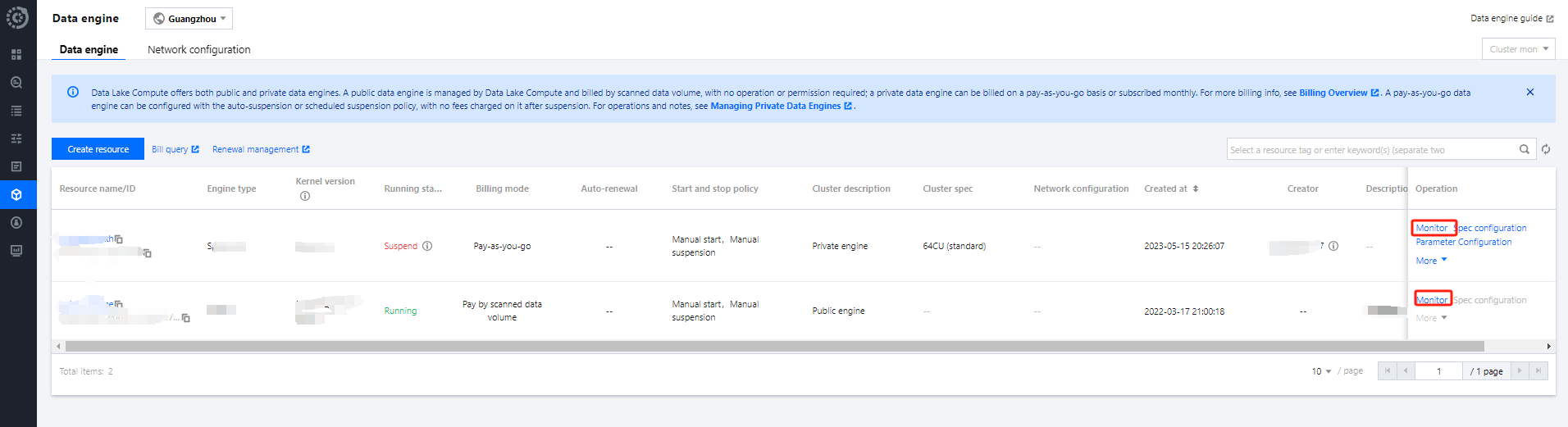
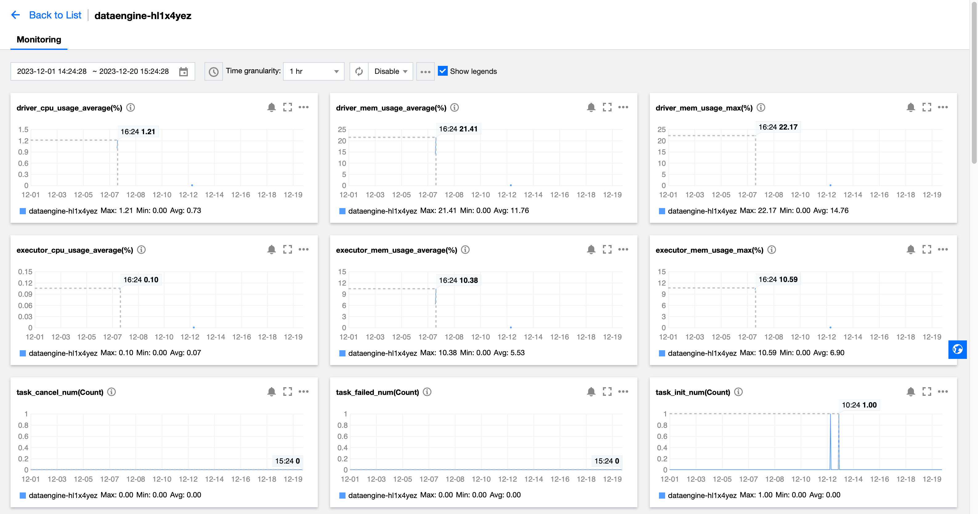
To assess whether resources have reached a bottleneck, DLC provides monitoring of engine resources such as CPU, memory, cloud disks, and network. You can adjust resource specifications according to business scale. For adjustments, refer to the Adjustment Configuration Fee Explanation. Steps to view engine resource usage are as follows:
1. Open the Data Engine Tag page on the left.
2. Click the Monitoring button on the right side of the respective engine.
3. Navigate to TCOP, where you can see all monitoring metrics as shown below. For detailed operations and monitoring metrics, refer to Data Engine Monitoring. You can also configure alarms for each metric. For a detailed introduction, refer to Monitoring and Alarm Configuration.
Other Factors
Adaptive Shuffle
DLC has Adaptive shuffle off by default. When your task encounters disk space insufficient issues like No space left, you can enable Adaptive shuffle, which supports regular shuffle with limited local disk space while ensuring stability in scenarios of large shuffle and data skew. Advantages of Adaptive Shuffle include:
1. Reduce storage cost: The disk mounting capacity of cluster nodes is further reduced, with general scale clusters requiring only 50G per node and large-scale clusters not exceeding 200G.
2. Stability: The stability of task execution for scenarios with a sharp increase in shuffle data volume or data skew will no longer fail due to limited local disk.
Although Adaptive shuffle brings cost reduction and stability improvement, in some scenarios, such as when resources are insufficient, it may cause about 15% delay.
Enable method:
The following configuration is added to the cluster configuration and enabled: spark.shuffle.manager=org.apache.spark.shuffle.enhance.EnhancedShuffleManager
Optional configuration:
If you wish to write data to the remote end in advance, underwrite sufficient disk space to avoid affecting other tasks, you can consider the following configuration:
spark.shuffle.enhanced.usage.waterLevel1=Disk ratio, the proportion of used Disk when writing shuffle results to the remote end, default 0.7.
spark.shuffle.enhanced.usage.waterLevel2=Disk ratio, the proportion of used disk space when shuffle spill data is written to the remote end, default 0.9.
Cluster cold start
The DLC supports the automatic or manual suspension of a cluster. After the suspension, no charges are incurred. Therefore, the message "Queuing" may be displayed when a task is executed for the first time after the cluster is started, because resources are being pulled up during the cold start of the cluster. If you submit tasks frequently, it is recommended to Purchase a package year/month cluster,which does not have a cold start and can quickly execute tasks at any time.
Iceberg
Partition Scan and Predicate Pushdown
In Spark + Iceberg scenarios, it is common to encounter deteriorating performance when reading partition tables due to oversized actual scan partitions (commonly used is scanning the entire table directly). The reason is that the scan condition for the partition field specified in the SQL where condition cannot be properly pushed down to the Scan operator, resulting in the need to scan the entire table first in Iceberg Scan and then apply filtering in Spark.
The performance in this type of scenario shows poor read table performance, with the Stage Input data volume in Spark UI far exceeding expected.
Common issues that cause this kind of filter condition predicate to fail to be pushed down to the operator include:
The partition field type and the constant value type specified in SQL are inconsistent.
The filter criteria specified in SQL perform function compute on the partition field, but Iceberg does not support this kind of function compute push down.
# ICEBERG TABLE partition_table PARTITIONED BY (dt STRING)## Predicate push down works normally, only scanning the partition file with dt='20260109'select * from partition_table where dt = '20260109';## Scenario 1: Because the data type is incorrect, the predicate cannot be pushed down, scanning all partitions.## Spark actually parses into select * from partition_table where cast(dt as int) = 20260109, but the cast operation is unsupported by Icebergselect * from partition_table where dt = 20260109;## Scenario 2: Because function compute is applied to the partition field, the predicate cannot be pushed down, scanning all partitions.select * from partition_table where date_diff(dt, '2026-01-08') > 7
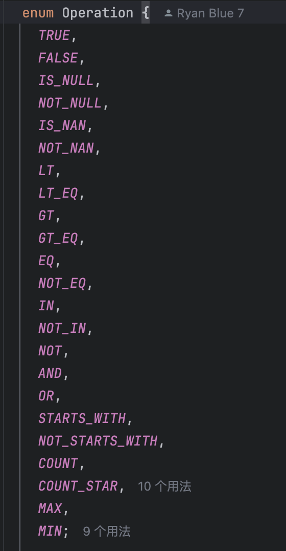
The partition field functions supported by ICEBERG for push down are limited to the following functions.
If your engine version was purchased before 2025-12-19, the above two scenarios would cause the predicate to fail to be pushed down, resulting in poor performance when Iceberg scans the entire table. At this point, you can only avoid this issue by modifying the SQL.
If your engine version was purchased after 2025-12-19, the field type mismatch between the constant value and partition field in scenario 1 will be optimized automatically. For scenario 2 with function compute, task-level parameters are controllable. The details of supported features in these scenarios are as follows.
Scenario 1
Scenarios with partition field and constant value, SQL such as where partition_filed OP Literal
For scenarios where OP is <=>, =, <=, >=, >, <, when the constant value type is inconsistent with the partition field type, it will automatically convert the constant value type to match the partition field type, format such as dt = cast (Literal as Type_Of_dt).
It can be controlled through the parameter spark.sql.optimizer.enableNormalizePartitionFilterCasts=true, true by default.
# ICEBERG TABLE partition_table PARTITIONED BY (dt STRING)## Predicate push down works normally, only scanning the partition file with dt='20260109'select * from partition_table where dt = '20260109';## Predicate push down works normallyselect * from partition_table where dt = 20260109;select * from partition_table where dt > 20260109;select * from partition_table where dt between 20260107 and 20260109;
Scenario 2
Scenarios with partition field involving function compute, SQL such as where function(partition_field) or where function(partition_field) = Literal
It can be controlled through the parameter spark.sql.optimizer.foldingPartitionFiltersInDatasourceV2=true, false by default.
This scenario takes effect with the following restrictions:
1. Restrictions on partition_field types: ShortType, IntegerType, LongType, FloatType, DoubleType, DecimalType, StringType, DateType, TimestampType, TimestampNTZType.
2. partition_field without switch: cannot include transformer, such as partitioned by year(dt), partitioned by bucket(6, dt)
3. function must be deterministic and a built-in function.
4. The total number of matched partition values for the function is less than or equal to 366. For multi-level partitioning, the total count here includes bottom-level partitions, such as year=2026&month=01 and year=2026&month=02 counted twice. You can adjust the number limit through the parameter spark.sql.optimizer.foldingPartitionFiltersMaxSize.
5. If matched to a null partition value, we will clarify to replace it with isNull(partition_field). Other null value scenarios are not supported.
6. The function can support a partition field as parameter, or both parameters for first-level partition and secondary partition. Other scenarios are not supported.
In addition, we have verified some common functions including date_diff, contains, concat, date_add, len, ends_with, unix_timestamp, date_format, coalesce, addition, subtraction, multiplication, and division. Other functions are under continuous verification. If you encounter any unsupported functions, please provide feedback to us.
# ICEBERG TABLE partition_table PARTITIONED BY (dt STRING)## Predicate push down works normally, only scanning the partition file with dt='20260109'select * from partition_table where dt = '20260109';## Predicate push down works normallyselect * from partition_table where date_diff(id, '2025-12-14') < 7;select * from partition_table where date_format(ds, 'yyyy-MM-dd') is null;select * from partition_table where unix_timestamp(ds, 'yyyy-MM-dd') >= unix_timestamp('2025-12-21', 'yyyy-MM-dd');# ICEBERG TABLE partition_table PARTITIONED BY (dt STRING, hour STRING)## Predicate push down works normallyselect * from partition_table where unix_timestamp(concat(dt, ' ', hour), 'yyyy-MM-dd HH') >= 176000000;
Help and Support
Was this page helpful?
You can also Contact sales or Submit a Ticket for help.
Help us improve! Rate your documentation experience in 5 mins.
Feedback